Simple Linear Regression Concept

Introduction

In today's highly competitive and rapidly evolving automotive industry, accurate sales forecasting has become a crucial aspect for manufacturers to stay ahead of the curve. This is particularly true for companies like Tesla, the leading producer of electric vehicles, which has gained widespread recognition for its innovative approaches and exponential sales growth. In this comprehensive blog post, we will delve into the application of Simple Linear Regression as a tool to forecast Tesla's vehicle sales in the United States.

To provide a thorough understanding, we will first explore the fundamental theoretical concepts of simple linear regression, which serves as the foundation for this forecasting technique. Following that, we will present a detailed, step-by-step Python implementation of the methodology, enabling readers to gain practical insights into the process. By the end of this blog post, you will have a solid grasp of how Simple Linear Regression can be effectively employed to predict Tesla's sales performance in the US market, and how this knowledge can be applied to other industries as well.

What is Simple Linear Regression?

A single dependent variable (in this case, sales) and a single independent variable (time or any other acceptable predictor) are modelled using the statistical technique known as simple linear regression. We can generate predictions based on past data since it implies a linear relationship between the two variables.

Dataset

We'll use a dataset with historical Tesla car sales information for the US in this presentation. Two columns should be available in the dataset: "Sales" (the number of automobiles sold in that particular month) and "Date," which represents time.

Date	No of Sales(units)
1/1/2022	100
2/1/2022	120
3/1/2022	130
4/1/2022	140
5/1/2022	160
6/1/2022	170
7/1/2022	190
8/1/2022	200
9/1/2022	210
10/1/2022	220
11/1/2022	230
12/1/2022	250
1/1/2023	260
2/1/2023	280
3/1/2023	290
4/1/2023	300
5/1/2023	320
6/1/2023	330
7/1/2023	340
8/1/2023	350

Step-by-Step Implementation

Import Required Libraries
```
 import pandas as pd
 import numpy as np
 import matplotlib.pyplot as plt
 from sklearn.linear_model import LinearRegression
```
Importing the essential Python libraries is the first step. 'LinearRegression' from 'sklearn.linear_model' was used to construct our regression model, along with 'pandas' for data processing, 'numpy' for numerical operations,'matplotlib' for data visualization, and 'numpy' for data handling.

Load and Prepare the Data

 # Load the dataset
 data = pd.read_csv('tesla_sales_data.csv')

 # Convert 'Date' column to datatime type
 data['Date'] = pd.to_datatime(data['Date'])

 # Sort the data based on 'Date'
 data.sort_values(by='Date', inplace=True)

 # Extract 'Date' as the independent variable (X) and 'Sales' as the dependent variable (Y)
 X = data['Date'].values.reshape(-1, 1)
 Y = data['Sales'].values.reshape(-1, 1)

To perform a time series analysis, we load the dataset and check that the 'Date' column is in the appropriate datetime format. Date is then extracted as our independent variable (X) and Sales are extracted as our dependent variable (Y) after sorting the data according to dates.

Split the Data into Training and Test Sets

 # We'll use the first 80% of the data for training and the last 20% for testing
 train_size = int(len(X) * 0.8)
 X_train, X_test = X[:train_size], X[train_size:]
 Y_train, Y_test = Y[:train_size], Y[train_size:]

To assess the effectiveness of our regression model, we separate the data into training (the first 80%) and testing (the last 20%) sets.

Create and Train the Linear Regression Model
```
 regressor = LinearRegression()
 regressor.fit(X_train, Y_train)
```
We set up the linear regression model and fit the practice data to it.
Make Predictions and Evaluate the Model
```
 Y_pred = regressor.predict(X_test)

 # Calculate Mean Squared Error
 mse = np.mean((Y_pred - Y_test) ** 2)
 print("Mean Squared Error:", mse)
```
Using the trained model, we make predictions on the test set and compute the Mean Squared Error (MSE) to evaluate the precision of our model's predictions.

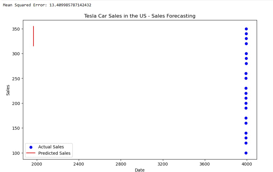
Visualize the Predictions

 plt.figure(figsize=(10, 6))
 plt.scatter(X, Y, color='b', label='Actual Sales')
 plt.plot(X_test, Y_pred, color='r', label='Predicted Sales')
 plt.xlabel('Date')
 plt.ylabel('Sales')
 plt.title('Tesla Car Sales in the US - Sales Forecasting')
 plt.legend()
 plt.show()

To demonstrate how well the model matches the data, we depict the actual sales data points and the line that represents the model's predictions.

Output

Conclusion

In this article, we have examined the application of Simple Linear Regression for forecasting Tesla car sales in the United States. We have provided a comprehensive, step-by-step Python implementation, encompassing data collection, preparation, and evaluation of the model's performance. Tesla and other automobile manufacturers can employ Simple Linear Regression to analyze their sales trends, thereby obtaining valuable insights to inform decision-making and facilitate strategic planning for the future.

Applying Simple Linear Regression to Predict Tesla Car Sales in the US